By: Kyra R. Shoemaker
Introduction
National infrastructure is one of the single most important things to determine the quality of life for any nation. It is how citizens eat, drink, travel, work. The USA Patriot Act, defined infrastructure as “systems and assets, whether physical or virtual, so vital to the United States that their incapacity or destruction would have a debilitating impact on national security, national economic security, national public health or safety, or any combination of those matters” (May & Koski, 2013). Therefore, the importance of infrastructure is that it keeps the nation running and operational for all levels of government, all private institutions, and every individual. If even one aspect of public infrastructure fails, millions of people will begin to suffer instantly.
According to a background written for The Council on Foreign Relations, “U.S. infrastructure is both dangerously overstretched and lagging behind that of its economic competitors” (McBride & Siripurapu, 2021). All forms of infrastructure, such as water, sewage, electricity, and transportation, require significant investment increases to keep them from failing and enhance the systems. Some lawmakers have offered proposals over the past several years to attempt to cover the gap and fix a broken financing system. They proposed increases in federal spending, a federal infrastructure bank, and public-private partnerships. Still, the most recent plan is a Congressional bill approved in November of 2021, which authorized a historic increase in spending on infrastructure by hundreds of billions of dollars (McBride & Siripurapu, 2021). However, it is sometimes bills or governmental actions like this that could cause blockages to infrastructure improvement.
One issue caused by infrastructure failures is federalism. In the United States, there are multiple levels of government, and each one has a different amount of control across physical and political boundaries. May and Kolski (2013) write that lawmakers must address overlapping authorities and jurisdictions to implement national risk reduction policies, such as improving or updating infrastructure. The problems, however, begin when policy goals between those agencies diverge. “Implementation gaps arise when actors at multiple levels of governance do not agree on the seriousness of a given problem or have differing ideas concerning the purpose of the policy” or how to solve the problem (May & Koski, 2013). Scholars believe that formal collaboration only occurs after a “sufficient community of interest” develops among relevant agencies and groups. This only forms a foundation for later efforts to occur; it does not cause or implement any changes to development efforts.
The use of the National Strategy for the Physical Protection of Critical Infrastructure and Key Assets and the U.S. Department of Homeland Security’s National Infrastructure Protection Plan was meant to delineate a plan and circumvent problems before they could occur. The documents clearly state that infrastructure is a concern for almost all communities of interest. Specifically, 18 sectors are identified: Agriculture and food; Banking and Finance; Chemical Facilities; Commercial Facilities; Communications; Critical Manufacturing; Dams; Defense Industrial Base; Emergency Services; Energy; Governmental Facilities; Healthcare and Public Health; Information Technology; National Monuments and Icons; Nuclear Reactors, Materials, and Waste; Postal and Shipping; Transportation Systems; and Water Systems. Nine federal agencies are called to act with augmentation from 36 more, all states, most municipalities, and 230 professional associations and trade groups (May & Koski, 2013). This plan creates a vast community of interest to focus on reaction, not necessarily prevention, of infrastructure deterioration. Preventative actions are encouraged, but these actors and agencies were chosen to respond if a catastrophic event occurs. Failure of agencies to react before catastrophic events is the main reason why they occur in the first place.
Of the 18 infrastructure sectors listed above, there are two significant concerns about infrastructure development and maintenance: economics and safety. Roadways are the system by which the physical side of the economy travels. If roads are nonexistent or rough that trade goods are damaged or delayed, the economy suffers. The current infrastructure systems were built decades ago, and the lack of adequate maintenance and upgrade funding has caused U.S. economic performance to suffer. The American Society of Civil Engineers calculated that the U.S. has an infrastructure gap of $2.6 trillion. An infrastructure gap refers to the current need for investments in infrastructure. This will cost $10 trillion worth of lost GDP by 2039 if the gap is not corrected. A 2019 Global Competitiveness Report from the World Economic Forum ranked the U.S. thirteenth for its poor infrastructure quality, down from fifth in 2002 (McBride & Siripurapu, 2021).
In 1998, the American Society of Civil Engineers (2021) started to compile an annual report card grading the state of U.S. infrastructure. These grades are based on several measurable conditions analyzed by the ASCE: capacity, condition, funding, future need, operation and maintenance, public safety, resilience, and innovation. Does the capacity of the infrastructure tool meet the needs of the consumer? What is the physical condition? Is it falling apart? How much funding is this infrastructure receiving and costing, and does it need more, or is it worth the current cost? Is it functional and consistently maintained? Is the public safe to use it, or is the infrastructure causing health crises? Can the infrastructure mechanisms withstand their own usage, or is there the potential for it to fall apart within the next year? Lastly, is the infrastructure improving in functionality, or is the system becoming more efficient?
This past year’s report left the nation’s total infrastructure with a C-, up from a D+ in 2017 and the highest grade since the inception of this concept. The ASCE determines this cumulative grade from seventeen categories: aviation, public parks, bridges, railroads, dams, roads, drinking water, schools, energy, solid waste, hazardous waste, stormwater, inland waterways, transit, levees, wastewater, and ports. Each category receives its own grade, the highest being a B for railways and the lowest being a D- in public transportation. This year, only five categories improved aviation, drinking water, energy, inland waterways, and ports – while just one grade decreased, bridges.
For 2021, road infrastructure received a flat D. Roads were frequently underfunded, with more than 40% of the whole system being in poor condition. Due to the underfunding at all levels of government, there has developed a growing backlog of rehabilitation and maintenance needs. Outdated roads have cost Americans about $1,000 a year in lost time value and fuel. Roads have also become more dangerous for pedestrians on adjacent sidewalks, with fatalities on the rise, and over 36,000 a year are dying in vehicle collisions (American, 2021). The infrastructure needs an update, especially with the current developments in electric vehicles and autonomous driving and delivery.
As for safety, the concerns surpass the problems found in road infrastructure. Civil engineers have warned that bridges are structurally insufficient and nearly on the verge of collapse. According to a study done by the Government Accountability Office, 10% of bridges in the U.S. are structurally deficient or physically failing, and 14% are functionally obsolete or unable to fulfill their intended purpose (McBride & Siripurapu, 2021). The same goes for the roads themselves and all other infrastructure in the U.S.; just look at their grades.
More specifically, road maintenance is assessed with three criteria: How much does it cost to keep the road usable; how much deterioration is occurring, and are the users comfortable, happy, safe, and able to access facilities from the roads they are using? Road deterioration itself is classified into four categories: historical conditions, pavement age, amount of passenger and freight loads combined with climate or environmental conditions, and pavement type, material, depth, and technique. These variables can be used to track and predict deterioration.
Historical conditions refer to the level of deterioration that occurs over time. Roads are expected to deteriorate at a similar rate each period. Similarly, pavement age predicts the amount of deterioration but also sets parameters for rehabilitation and patches. If a pothole is filled, there is a separate deterioration calculation for the road, patch, and combined materials. Next, road usage, wear and tear, and the environment are all factors that cause pavement to degrade. Traffic volume, vehicle mass, speed and braking variability, temperature changes, weather patterns, surface evaporation, and flora and fauna break down the materials used unceasingly.
A study of roads in Western Australia authored by Song, Wu, Li, Liu, and Karunarante (2021) revealed that pavement significantly becomes rougher with age. From 0 to 40 years, roughness increased by 25% and grew to 60% by age 60 when no maintenance was performed. Effectively, the estimated end of usable life for a non-maintained road network is 63 years, after which the roughness of the road makes it nearly unusable for individual and commercial travel. Considering that most of the current infrastructure in the U.S. was designed and built in the 1960s, that lifespan is ending now (McBride & Siripurapu, 2021). This study also showed that the top five causes of deterioration are ranked as follows: temperature, deep water drainage, percentage of heavy vehicles, traffic volume, and soil moisture levels. The correlation between road roughness and pavement age was found to be 0.449 out of 0.1, while the correlation between roughness and the deteriorating factors was 0.705 out of 0.1 (Song et al., 2021).
One common way to measure the physical roughness of the road is through the International Roughness Index (IRI). The IRI is a measure of how rough or smooth the pavement is. One way to measure the IRI is by driving a specially equipped vehicle along the road to be measured. This vehicle would have a device installed that is capable of measuring the longitudinal movement of the suspension; how much the suspension of the vehicle moves up and down. The IRI is calculated by dividing the sum of the suspension motion by the length of the pavement section driven, usually recorded as m/km or in/mi. Typically, newly paved roads will be rated between 0.810 and 1.030 m/km, about 51.322 to 62.261 in/mi; smaller ratings have also been reported. The rating all depends on the type of pavement, quality of construction, and slope of the road itself (Piryonesi & Tamer, 2021). According to the Bureau of Transportation Statistics (BTS) (2022), an IRI rating of less than 95 is good, 95 to 170 is fair, and greater than 170 is poor. The higher the number, the rougher the roads. To receive a mark of “acceptable,” roads must have an IRI of 170 and less.
Literature Review on Response time
This half of the literature involves the length of time for police officers to arrive on the scene after a call for service is received.[1] However, there is very little research on the physical barriers to swift police response. Previous research typically looks at the distance to the call location from the nearest sub-station (Vidal & Kirchmaer, 2018; Clark et al., 2021; Simpson & Orosco, 2021; Lee et al., 2016), but nothing has questioned the physical environment the officers must traverse in order to reach the call location. Research generally focuses on the theories behind police response perception, the influence dispatchers have over the priority of calls made, and how many officers are needed to maintain or improve response times.
When Vidal and Kirchmaer (2018) studied the long-held belief that response time has no effect on arrest rates, it was determined that an increased response time of 10% actually decreases the likelihood of a crime being cleared at 4.7%. These authors determined that the initial response to a call for service is one of the most important parts of a criminal investigation. Arriving on the scene as quickly as possible increases the likelihood of finding witnesses and increases the clarity of their memories. It allows the officer to collect and preserve more evidence. Thus, a fast response time is a desirable goal for any police department, but what are other issues that affect an officer’s initial response time?
There are theories that attempt to explain the differences in response times for various communities, and these theories focus on social disorganization[2]. The ecological theory looks very specifically at the locality of the call for service; it says that officers responding to an area of high social disorganization will believe that the line between offender and victim is blurred. Therefore believing that the victim is less deserving of fast and decisive response (LaBerge, et al., 2022). Under this theory, as criminal activity in an area increases, perceived deservedness decreases. Luckily, studies have found this theory to be false (LaBerge et al., 2022). Ecological studies of social disorganization and response time show that officers tend to respond faster in areas with higher crime rates.
Studies questioning the influences on response time determined that ecological factors significantly affect the timeline of response. It was discovered that response times were shorter in neighborhoods with large minority populations and a relatively small income compared to their population size. In this study, researchers hypothesized that this might be caused by a higher volume of calls for service in the area, so patrols were pre-staged as a part of strategic planning. Further studies confirmed this hypothesis. Strategic and tactical planning has become a large part of police administration duties. Commanders and chiefs have seen this research and determined that to help their communities and suppress criminal activity, they must target high-crime rate areas with more police presence (Lee et al., 2016). Response times have decreased, but some citizens worry that minority populations are being targeted.
Potential personal bias is a far more compounding problem when it comes to the length of response time. Dispatchers have a lot of influence over the response time and order for calls. Each call is given a call type and a priority number. Call types determine the kind of call for service received: homicide, assault, robbery, etc. Priority numbers determine what order the calls should be responded to, which request is more urgent than others, and which call is in progress and could potentially be stopped with the offender on scene. Researchers wanted to know if the bias and unintentional priming from the dispatcher impacted an officer’s response time. LaBerge, Mason, and Sanders (2022) showed that dispatchers prioritized or unintentionally encouraged officers to respond to areas with high residential instability, but not necessarily areas with concentrated economic or social disadvantage.
Police response time is heavily influenced by perceptions of officers and dispatchers. However, what are the physical influences on travel time for officers once they receive a call for service? How much influence does a $2.6 billion infrastructure maintenance gap have over the terrain officers must travel to reach call locations? The following research intends to answer this question: what is the relationship between deteriorating road infrastructure and emergency response time? The current hypothesis: as the number of deteriorated miles increases in urban areas, the number of seconds in the response time increases.
Research Design
Using the IBM Statistical Package for the Social Sciences (SPSS) software, road infrastructure deterioration will be compared to emergency response time. The independent variable will be road infrastructure deterioration, based on its viability or roughness rating known as the International Roughness Index (IRI). The dependent variable will be response time, based on the number of seconds elapsed between an initial call for service and the first responder to arrive on the scene. To determine if these two variables are related, correlation testing will be used.
Data
First, data detailing the current viability and usability of public roads was gained from the Bureau of Transportation Statistics (BTS), a department of the United States Department of Transportation. The data table used is known as Road Condition and falls under State Transportation Statistics (Bureau, 2022). This table holds data that compares the International Roughness Index (IRI) of each state’s roads divided into two categories, urban and rural roads. These two categories are further divided into the types of roads analyzed (Other Principal Arterials; Other Freeways; Expressways; Minor Arterial; Major and Minor Collector; and Interstate), and, of course, the total miles and total acceptable miles according to the IRI. A rating of less than 95 is good, 95 to 170 is fair, and greater than 170 is poor. For this data table, the BTS has stated that “acceptable” miles have an IRI of 170 and less. The IRI has been published 17 times; in 1995, 2000, from 2005 to 2009, and from 2011 through to 2020 (Bureau, 2022).
The second source of data comes directly from police departments. Data gathered from this source were the response times reported in calls for service datasets. ‘Calls for service’ is the technical term for all calls received by a dispatching department and is usually collected by a Computer-Aided Dispatch (CAD) system. Each police department uses these systems and terms differently; however, the most general system will capture requests made from “emergency 911 phone calls, non-emergency phone calls or text messages, officer self-initiated, and alarms” (Chandler, 2022). This data was harder to find because this information is self-reported data not required by any centralized agency.
The Police Data Initiative, founded in 2017, is a community of 120 law enforcement agencies that have preemptively decided to follow the recommendations of the Task Force on 21st Century Policing. The task force focused on technology and transparency (National, 2022). Of the 120 law enforcement agencies participating in the Police Data Initiative, 21 submitted datasets regarding their calls for service; of the 21, 4 included the number of seconds between the time of the call and responder arrival time (National, 2022). Those four departments are the Chandler Police Department in Chandler, Arizona starting in 2016; the Mesa Police Department in Mesa, Arizona starting in 2017; the Montgomery County Police Department in Gaithersburg, Maryland starting in 2017; and the Portland Police Bureau in Portland, Oregon starting in 2012 (Chandler, 2022; Police, 2022; Montgomery, 2022; Police Bureau, 2022).
Data Manipulation
Due to the lack of a large body of published response time data, this study will not make conclusions about the effect of road deterioration on response time in the entirety of the United States of America. The data gathered will be analyzed in a small number of case studies. The same processes and analyses are performed in each case. As stated earlier, it was found that only four law enforcement agencies published the number of seconds it took for a first responder to arrive on the scene; each agency will be one case study. Of course, each agency had labeled and collected its data differently. Thus, the first act performed on the data was to homogenize the variables. Each agency was condensed to three variables: agency name, year of call, and the response time in seconds.
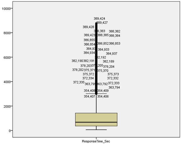
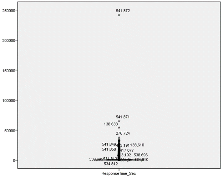
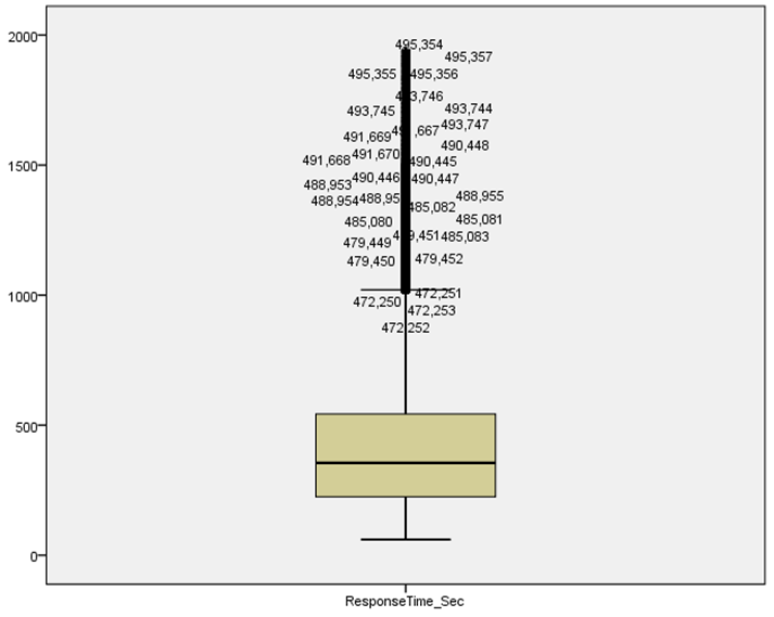
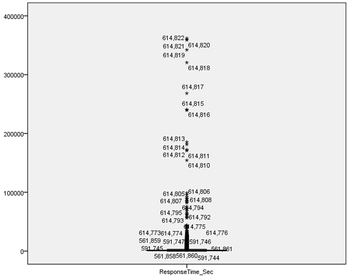
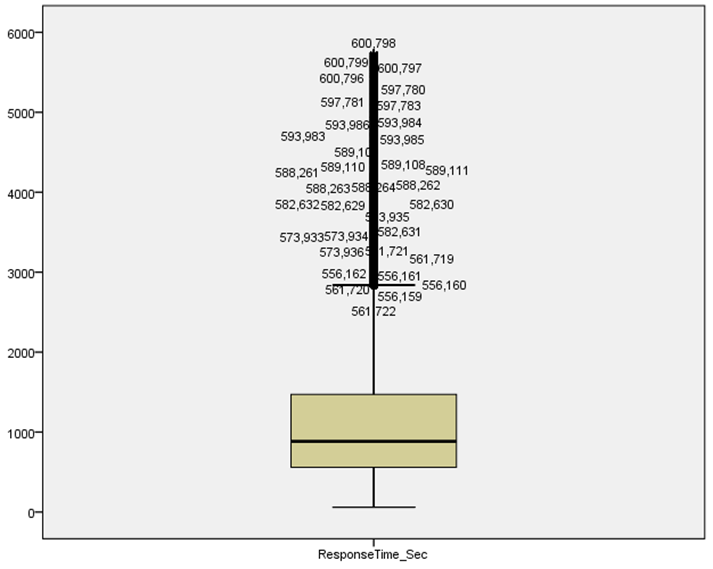
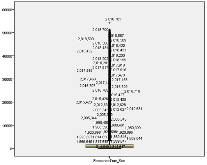
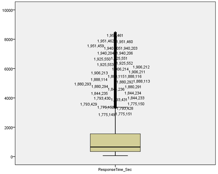
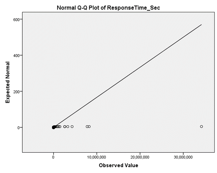
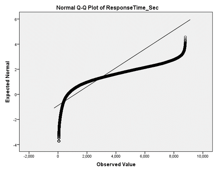
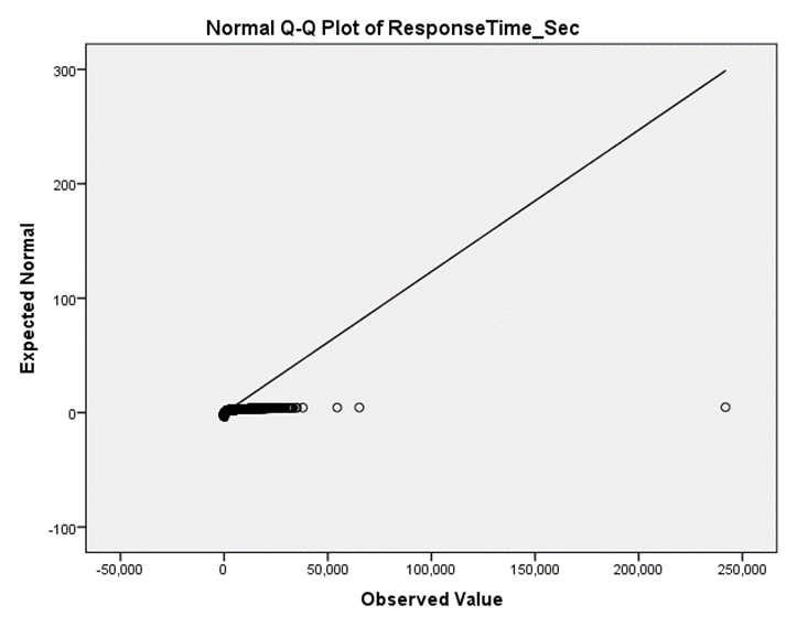
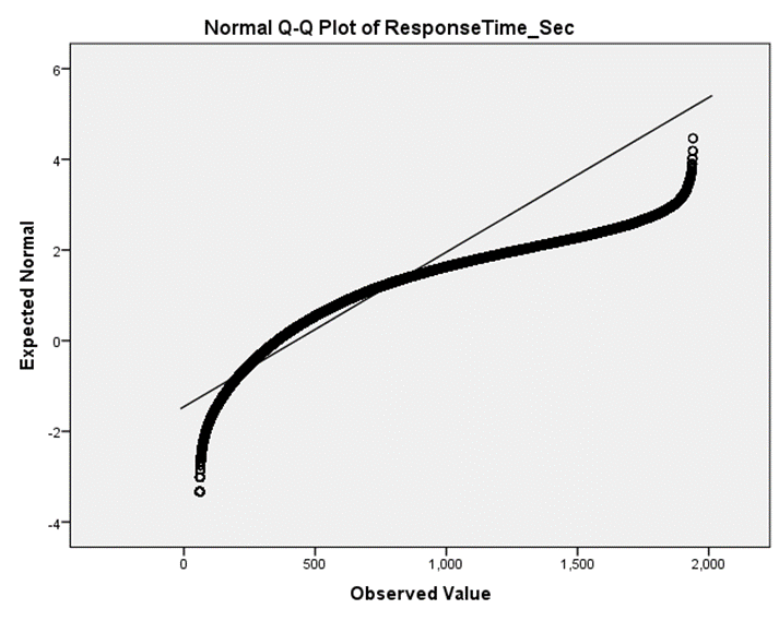
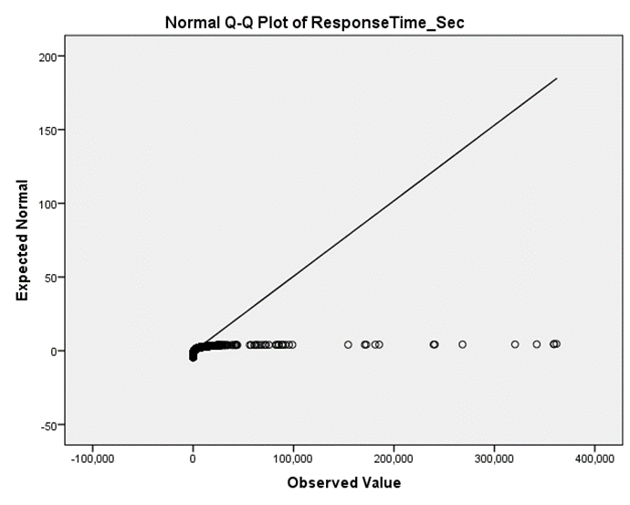
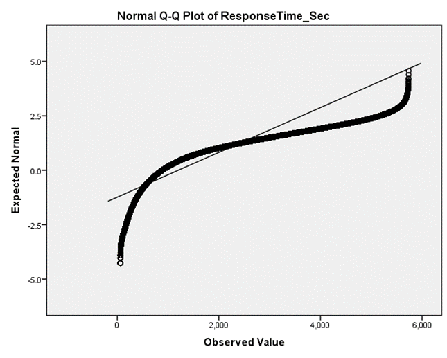
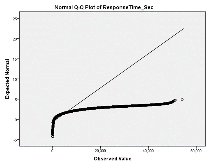
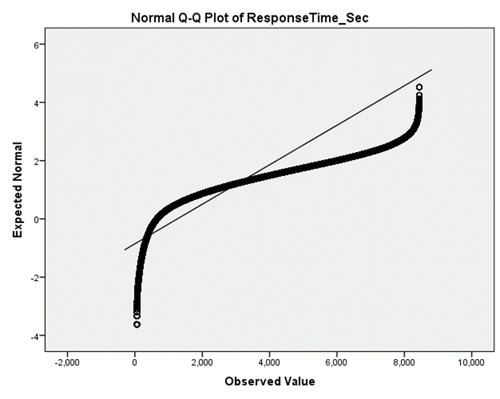
Once condensed, all response times taking less than 60 seconds were removed to correct for officer-initiated calls for service, such as traffic stops, spot searches, and in-person requests for emergency action. There is an option in some of the databases to remove officer-initiated calls. This option was not used because it would also remove officer requests for backup. The reason for removing data where the response was less than 60 seconds was to be sure that the person responding had to travel from one spot to another and had the potential to use roads for that. Removing officer-initiated calls would have removed more data than necessary. The next step taken for the response time data was to remove the outliers. The longest 2% of response times were removed from the analysis. This was to protect the analysis from the potential human error where the responders forgot to stop the timer for their arrival on the scene. See appendices A through D for the before and after outlier charts of removing the less than 60 seconds and longest 2% data. See appendices E through H for the Normal Q-Q Plot, showing the expected normalcy of the data before and after removing the outlier data.
Similar changes must also be made to the Road Conditions data from the BTS. The IRI data in this table was divided into urban and rural roads. Only the data on urban roads was used because all the agencies in the case studies operated out of highly populated areas and medium to large cities. It was separated again into the types of roads: interstate, major and minor collectors, minor arterial, other freeways and expressways, and other principal arterials. Each road type was then divided again into the number of miles per IRI score: less than 60, 60 to 94, 95 to 119, 120 to 144, 145 to 170, 171 to 194, 195 to 220, and more than 220. The only exceptions to this division were the minor arterial and the major and minor collector data, where the 171 to 194 and the 195 to 220 categories were combined in the original data (Bureau, 2022). Each of these categories were simplified for the case studies. The IRI scores were divided into acceptable and unacceptable categories based on the BTS’s measure that an IRI of 170 and less was acceptable. The IRI scores for each road type were then combined to make the ‘total miles acceptable’ and a ‘total miles unacceptable’ category for all urban roads. This process was applied to the Road Condition data tables from the three states where the response time data was gathered: Arizona, Maryland, and Oregon. This data was sorted by the year it was collected and allowed for the IRI data to be compared with more detail to the response time data, which had also been sorted by year.
Methods
The response time in seconds from each agency was then analyzed against the IRI data from their respective state. Correlation testing was used for this analysis. Correlation is a statistical technique used to show if two variables are mathematically associated and how strong the association is or the degree to which they are associated. The strength of the correlation is determined by the correlation coefficient, which runs from 1 to -1. Positive correlation determines that both variables move in the same direction, increasing or decreasing with each other. A negative correlation is where the variables move in opposite directions at the same time; as one increases, the other decreases at a similar rate. A perfect correlation, where the coefficient is either 1 or -1, shows that the variables change at the same ratio or rate. A high degree of correlation has a correlation coefficient of 0.75 or higher, moderate is between 0.50 and 0.75, low correlation is between 0.25 and 0.50, and an absence of correlation is between 0.00 and 0.25. Significance is also important while calculating the degree of correlation; it is what determines the odds of the correlation occurring simply by chance. The significance test used for this research is a two-tailed test. In this type of test, the desired outcome is a significance equal to or less than 0.01, meaning the odds that the correlation coefficient occurred by chance are 1 out of 100. The last calculation is the coefficient of determination. This is the measurement of the variance caused by one variable’s relationship with another variable (Complete, 2022).
Correlation tests use two types of hypotheses, null and alternative. A null hypothesis states that there will be no correlation between the variables being tested. An alternative hypothesis states that there will be a correlation present. Thus, the null hypothesis for this research is that there is no correlation between the deterioration of road infrastructure and emergency response time. The alternative hypothesis states that there is a correlation between the two variables. That response time is affected by decreasing IRI. To run the correlation calculations for these hypotheses, SPSS was used, and the correlation tables can be found in appendices I through L.
Results
First, the correlation table for the relationship between the Chandler Police Department in Arizona and the number of unacceptable urban miles in Arizona, as determined by the IRI between the years 2016 and 2020. The significance for this correlation was 0.000, meaning that there is a nearly non-existent chance that the relationship between the variables is random. The correlation coefficient is -0.017, meaning that the relationship is negative (see appendix I). However, the coefficient does not meet the 0.25 threshold and is, therefore, absent. The strength of determination would have been 0.000289. For the case of the Chandler Police Department, the null hypothesis is accepted; there is no correlation between road deterioration and response time.
Second, the correlation table for the relationship between the Mesa Police Department in Arizona and the number of unacceptable urban miles in Arizona, as determined by the IRI between the years 2017 and 2020. The significance for this correlation was also 0.000, meaning there is very little chance the relationship is random. The correlation coefficient is 0.009, and the relationship is positive (see appendix J). However, it does not meet the threshold, and correlation is assumed to be absent. The strength of determination would have been 0.000081. The null hypothesis is accepted for the Mesa Police Department analysis.
Third, the correlation table for the relationship between the Montgomery County Police Department in Maryland and the number of unacceptable urban miles in Maryland, as determined by the IRI between the years 2017 and 2020. The significance for this case is also 0.000; the relationship is not random. The correlation coefficient is -0.022; the correlation is negative and does not meet the required limit; correlation is considered to be absent (see appendix K). The coefficient of determination would have been 0.000484. The null hypothesis is accepted for the Montgomery County Police Department in Maryland.
Fourth, the correlation table for the relationship between the Portland Police Bureau in Oregon and the number of unacceptable urban miles in Oregon, as determined by the IRI between the years 2012 and 2020. The significance for this case is 0.000; the relationship would not be considered chance. The correlation coefficient is -0.12, a negative relationship, and below the correlation threshold, the correlation is absent (see appendix L). The coefficient of determination would have been 0.000144. For the case of the Portland Police Bureau of Oregon, the null hypothesis is accepted.
Findings and Discussion
All four case studies held statistical significance but did not meet the minimum standard for correlation; thus, the numbers imply that the physical condition of the roads does not have an impact on emergency response time. This begs the question, why would these seemingly logically connected variables not have a statistical relationship? The answer to this question falls into two categories, the data itself and outside influences.
Looking at the IRI itself, it only allows for the influence of the road’s physical condition. There is no accounting for the influence of infrastructure functionality on increased traffic in urban areas and no way to measure its effect on response time. The outside influences on the data revolve around the police themselves. Since officers typically live near the areas they work in, and many officers stay with the same department their whole career, they might just know their patrol areas so well that whatever time incurred by deteriorated roads is negated by their traffic knowledge. Maybe officers are not concerned with wear and tear to their patrol vehicles and costs for maintenance, so they simply drive over the rough roads. There is potential that the lights and sirens officers can use to split traffic negate any time difference caused by roughness. These ideas are conjecture, but there are two measurable outside influences already cited in this paper that might be reasons the response time is not affected by increased deteriorated IRI miles.
Potentially, officers already being present in deteriorated areas, which are typically economically depressed areas, negate road deterioration; or the number of officers on patrol. A technique used to prevent and react to crime quickly is strategic planning. Police Chiefs and commanders use these plans to place officers and patrols in areas with statistically more instances of crime. To stop crime as it occurs, patrols are located where criminal actions are most likely to occur (Lee et al., 2016). If officers are already in or near the areas where crimes are occurring, the travel distance is short enough that bad roads affect response time minimally. The same reasoning applies to the workforce. If there are an overwhelming number of officers in the high crime areas, there are more officers able to respond, meaning that there is a higher chance that someone is nearby and able to respond quickly. Referring to the study done on the city of Chicago, the police department could lose almost 40% of its workforce to new personnel, and it would still maintain its current response times (Clark et al., 2021).
Also, an interesting observation to note is that the correlation for three out of the four cases, if the correlation was statistically defensible, is negative. A negative correlation implies that as the number of deteriorated roads increases, the amount of time it takes for an officer to respond decreases. Simply, the worse the roads are, the faster officers respond. If this were true, strategic planning could possibly be praised as being able to negate any time incurred due to bad roads.
Limitations and Recommendations
The major limitations to this research were potential human error, a minimal variety of response time data, and the length of data collection. In the call for service data published by the Chandler, Arizona police department, the single longest response time to be deleted as an outlier added up to 395.96 days. The call was in response to a “city violation.” The second-longest response time from Chandler PD was 95.31 days, and this was a call for the Phoenix Fire Dispatch. Both of these calls were cleared with no contact, meaning that no contact was made with the originator of the call (Chandler, 2022). The problem this causes, even once these outliers are removed, is the potential that these calls are the product of human error in the response time system. What if the only reason the first call took over a year to gain a response was simply that the responders on the scene forgot to stop the clock? This is an example of human error being a manipulating limit on this research.
Data variety limited the number of police departments this study was able to analyze to determine how road roughness affected response time. Of the nearly 18,000 police departments in the U.S., only 26 were found to report their response time data, and then only four published the amount of time it took for someone to arrive on the scene (USA, 2021; National, 2022). As with all research, the results improve and are more accurate when more data exists. The same applies to the length of time the response time data has been collected. The Portland Police Bureau had the longest publication history, starting in 2012, making eleven years of data (Police Bureau, 2022). The Chandler Police Department started in 2016 (seven years), and the Mesa Police Department and the Montgomery County Police Department started in 2017 (six years) (Chandler, 2022; Police, 2022; Montgomery, 2022). However, IRI data was last published in 2020, meaning there were only nine years of overlapping data for the Portland Police Bureau, with the Chandler Police Department having five years and the Mesa and Montgomery County Police Departments having four (Bureau, 2022).
It is because of this limited time span that the first recommendation for future research is simply to wait for more time to pass. A few years down the line, it will be interesting to see if or how the correlation data changes. Also, attempt to find specific IRI data for the cities where the police departments are being studied. The IRI data used in this study was for urban miles of each state as a whole; maybe a city-specific IRI rating will yield different results. The last two recommendations attempt to treat the outside influences of the limitations of the data. First, it would help the data to find a way to study how traffic affects response time, not just the physical conditions of the roads. Also, study the effects of officer behavior on response time. Do officers know the roads so well they avoid all the roughness? Do they not have concern for the wear and tear on their vehicles caused by rough roads?
Conclusion
As discussed in previous literature, response time is a clear indicator of police performance in its community. A good response time increases community satisfaction and the likelihood of crime clearance. Also, road deterioration is a detriment to public health and safety; at the same time, it causes major harm to the nation’s economic growth. Despite there being no statistical correlation between these two variables, it would be in the best interest of lawmakers and law enforcers to have road infrastructure deterioration and emergency response time as parts of their national improvement plans.
References
American Society of Civil Engineers. 2021. “2021 Report Card for America’s Infrastructure.” American Society of Civil Engineers, Vol. 23.
Bureau of Transportation Statistics. 2022. “Road Condition.” United States Department of Transportation. https://www.bts.gov/road-condition (last visited April 28, 2022).
Chandler Police Department. 2022. “Calls For Service.” Chandler Police Department. https://data.chandlerpd.com/catalog/calls-for-service/ (last visited April 28, 2022).
Clark, Callie, Chitra Dangwal, Dylan Kato, and Marta Gonzalez. 2021. “A Network Spatial Analysis Simulating Response Time to Calls for Service at Variable Staffing Levels: A Study on Strategic Police Defunding in the City of Chicago.” The European Physical Journal: Special Topics, (December): 1-9.
Complete Dissertation. 2022. “Correlation in SPSS.” Statistics Solutions. https://www.statisticssolutions.com/correlation-in-spss/ (last viewed May 3, 2022).
LaBerge, Alyssa, Makayla Mason, and Kaelyn Sanders. 2022. “Police Dispatch Times: The Effects of Neighborhood Structural Disadvantage.” Journal of Criminal Justice, Vol. 79 (March): 1-9.
Lee, Jae-Seung, Jonathan Lee, and Larry T. Hoover. 2016. “What Conditions Affect Police Response Time? Examining Situational and Neighborhood Factors.” Police Quarterly, Vol. 20, No. 1 (July): 61-80.
May, Peter J., and Chris Koski. 2013. “Addressing Public Risks: Extreme Events and Critical Infrastructures.” Review of Policy Research, Vol. 30, No. 2 (March): 139-159.
McBride, James, and Anshu Siripurapu. 2021. “Backgrounder: The State of U.S. Infrastructure.” Council on Foreign Relations. https://www.cfr.org/backgrounder/state-us-infrastructure (last visited on May 7, 2022).
Montgomery County, MD. 2022. “Police Dispatched Incidents.” Montgomery County, MD. https://data.montgomerycountymd.gov/Public-Safety/Police-Dispatched-Incidents/98cc-bc7d (last viewed April 28, 2022).
National Policing Institute. 2022. “Police Data Initiative.” National Policing Institute. https://www.policedatainitiative.org/ (last visited April 28, 2022).
Piryonesi, S. Madeh, and Tamer E. El-Diraby. 2021. “Examining the Relationship Between Two Road Performance Indicators: Pavement Condition Index and International Roughness Index.” Transportation Geotechnics, Vol. 26, (January): 1-6.
Police Bureau. 2022. “Dispatched Calls For Service.” The City of Portland, Oregon. https://www.portlandoregon.gov/police/76454 (last viewed April 28, 2022).
Police, City of Mesa. 2022. “Police Computer Aided Dispatch Events.” Mesa AZ: Smart City. https://data.mesaaz.gov/Police/Police-Computer-Aided-Dispatch-Events/ex94-c5ad (last viewed April 28, 2022).
Simpson, Rylan, and Carlena Orosco. 2021. “Re-assessing Measurement Error in Police Calls for Service: Classifications of Events by Dispatchers and Officers.” PLoS One, Vol. 12, No. 12 (December): 1-19.
Song, Yongze, Peng Wu, Qindong Li, Yuchen Liu, and Lalinda Karunaratne. 2021. “Hybrid Nonlinear and Machine Learning Methods for Analyzing Factors Influencing the Performance of Large-Scale Transport Infrastructure.” IEEE Transactions on Intelligent Transportation Systems (September): 1-14.
USA Facts. 2021. “Police Departments in the U.S.: Explained.” USA Facts. https://usafacts.org/articles/police-departments-explained/ (last visited May 4, 2022).
Vidal, Jordi Blanes I, and Tom Kirchmaer. 2018. “The Effects of Police Response Time on Crime Clearance Rates.” Review of Economic Studies, Vol. 85, No. 2 (April): 855-891.
[1] A ‘call for service’ is the term used for when a civilian makes a call to a police dispatcher to request a police presence.
[2] Social disorganization refers to community characteristics like poverty, resident instability, racial and ethnic heterogeneity, and delinquency rates.
Appendices
Appendix A
Chandler Police Department outlier chart, including outliers
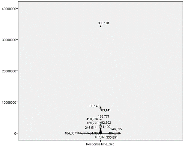
Chandler Police Department outlier chart, without outliers
Appendix B
Mesa Police Department outlier chart, including outliers
Mesa Police Department outlier chart, without outliers
Appendix C
Montgomery County Police Department outlier chart, including outliers
Montgomery County Police Department outlier chart, without outliers
Appendix D
Portland Police Bureau outlier chart, including outliers
Portland Police Bureau outlier chart, without outliers
Appendix E
Chandler Police Department, Normal Q-Q Plot of Response Time, with outliers
Chandler Police Department, Normal Q-Q Plot of Response Time, without outliers
Appendix F
Mesa Police Department, Normal Q-Q Plot of Response Time, with outliers
Mesa Police Department, Normal Q-Q Plot of Response Time, without outliers
Appendix G
Montgomery County Police Department, Normal Q-Q Plot of Response Time, with outliers
Montgomery County Police Department, Normal Q-Q Plot of Response Time, without outliers
Appendix H
Portland Police Bureau, Normal Q-Q Plot of Response Time, with outliers
Portland Police Bureau, Normal Q-Q Plot of Response Time, without outliers
Appendix I
Chandler Police Department Correlations Test
| Correlations | |||
| ResponseTime_Sec | UrbanMiles_TotalMiles_171AndMore_Unacceptable | ||
| ResponseTime_Sec | Pearson Correlation | 1 | -.017** |
| Sig. (2-tailed) | .000 | ||
| N | 389756 | 389756 | |
| UrbanMiles_TotalMiles_171AndMore_Unacceptable | Pearson Correlation | -.017** | 1 |
| Sig. (2-tailed) | .000 | ||
| N | 389756 | 389756 | |
| **. Correlation is significant at the 0.01 level (2-tailed). | |||
Appendix J
Mesa Police Department Correlations Test
| Correlations | |||
| ResponseTime_Sec | UrbanMiles_TotalMiles_171AndMore_Unacceptable | ||
| ResponseTime_Sec | Pearson Correlation | 1 | .009** |
| Sig. (2-tailed) | .000 | ||
| N | 496185 | 496185 | |
| UrbanMiles_TotalMiles_171AndMore_Unacceptable | Pearson Correlation | .009** | 1 |
| Sig. (2-tailed) | .000 | ||
| N | 496185 | 496185 | |
| **. Correlation is significant at the 0.01 level (2-tailed). | |||
Appendix K
Montgomery County Police Department Correlations Test
| Correlations | |||
| ResponseTime_Sec | UrbanMiles_TotalMiles_171AndMore_Unacceptable | ||
| ResponseTime_Sec | Pearson Correlation | 1 | -.022** |
| Sig. (2-tailed) | .000 | ||
| N | 601919 | 601919 | |
| UrbanMiles_TotalMiles_171AndMore_Unacceptable | Pearson Correlation | -.022** | 1 |
| Sig. (2-tailed) | .000 | ||
| N | 601919 | 601919 | |
| **. Correlation is significant at the 0.01 level (2-tailed). | |||
Appendix L
Portland Police Bureau Correlations Test
| Correlations | |||
| ResponseTime_Sec | UrbanMiles_TotalMiles_171AndMore_Unacceptable | ||
| ResponseTime_Sec | Pearson Correlation | 1 | -.012** |
| Sig. (2-tailed) | .000 | ||
| N | 1959169 | 1959169 | |
| UrbanMiles_TotalMiles_171AndMore_Unacceptable | Pearson Correlation | -.012** | 1 |
| Sig. (2-tailed) | .000 | ||
| N | 1959169 | 1959169 | |
| **. Correlation is significant at the 0.01 level (2-tailed). | |||