Nicholas Unger
The United States’ policies on alcohol are a widely debated topic of discussion; however, empirical research on the effectiveness of state alcohol regulations through state-to-state comparison is insufficient. This study answered whether or not stricter alcohol laws positively impact public health and safety by comparing and analyzing the alcohol laws of California and Pennsylvania, with a direct focus on what said laws have on each state’s public health and safety. Moreover, these states were chosen for this study due to the significant differences in the overall strictness of their alcohol laws. To specify, California held more lenient alcohol restrictions while Pennsylvania is among one of the states with the most regulations on alcohol. This study aimed to determine whether or not strict alcohol regulations helped prevent alcohol-related fatalities and harm.
A comparison between the alcohol-related abuse and harm data from both California and Pennsylvania determined the effects that these laws have concerning public health and safety. In doing so, this study determined that more liberal access to alcohol increases the risks to the public’s health and safety, for example, looking into cases of drunk driving, alcohol addiction, or deaths related to alcohol. The results of this study contribute valuable insights into whether a more liberal or conservative approach to alcohol legislation is more effective in safeguarding public health and reducing alcohol-related harms. Thus, this study demonstrated that California—providing more liberal accessibility to alcohol—holds higher rates of alcohol-related harms than its counterpart, Pennsylvania; an argument can be made to enact more regulations in the name of public health and safety.
Literature Review
Previous research articles that directly relate to this study have analyzed the relationship between alcohol availability and alcohol consumption, U.S. alcohol policy and how it affects binge drinking, as well as the effects of alcohol access laws on highway safety. This study served as a significant benefit to this research through an analysis of the effects of alcohol laws on highway/traffic safety and binge drinking. In doing so, this research covered these critical aspects of alcohol-related harms that still require more in-depth research rather than solely analyzing alcohol consumption. The individual harms of alcohol consumption, such as traffic incidents, deaths, and binge drinking, were analyzed in order to accurately depict how alcohol policy is affecting public health and safety. Thus, it warrants further research due to the lack of a comprehensive state alcohol policy comparison.
In the article of the American Journal of Preventative Harms titled “The Effectiveness of Limiting Alcohol Outlet Density As a Means of Reducing Excessive Alcohol Consumption and Alcohol-Related Harms,” by Carla Alexia Campbell, Robert A. Hahn, Randy Elder, et al., the researchers aimed to find out whether limiting alcohol outlet densities effectively prevent alcohol consumption and related harms. In their tests, they considered policies such as privatization, liquor by the drink, and bans, which affected alcohol availability. These researchers claim that their tests showed evidence that policies that reduce alcohol outlet density actually reduce excessive alcohol consumption and alcohol-related harms. Therefore, it is logical to assume that these policies can help address the amount of consumption and, in return, would help prevent alcohol-related harms. Furthermore, the authors theorized that “[o]utlet density is hypothesized to affect excessive alcohol consumption and related harms by changing physical access to alcohol (i.e., either increasing or decreasing proximity to alcohol retailers), thus changing the distance that drinkers need to travel to obtain alcohol or to return home after drinking” (Campbell, et al. 557). The methods used in this study is that of the Community Guide process, executed by a series of analysis involving a review development team which then decides whether evidence is applicable to the hypothesis. If the evidence has validity, then it is taken to the Task Force on Community Preventive Services. This independent scientific review board reviews the evidence and determines if it is enough to suggest new recommendations for prevention tactics. For this study, both time series and cross-sectional studies were used to determine the effectiveness of limiting alcohol outlet density on alcohol consumption and related harms. The results of these studies found that “most of the studies included in this review reported that greater outlet density is associated with increased alcohol consumption and related harms, including medical harms, injuries, crime, and violence” (Campbell et.al 565-566). The results of their studies confirmed the researcher’s original hypothesis. There are several research gaps that the authors mention that warrant further research, one of which is the economic impact of limiting alcohol outlet densities. Due to this, future research endeavors could delve deeper into the economic ramifications of decreased alcohol outlet densities, providing a more comprehensive understanding of the multifaceted impact of alcohol policies. Another gap in the research is the lack of studies that evaluate local policies affecting alcohol outlet density and its effects. The effects that alcohol laws have on consumption are also researched and described by authors Stanley I. Ornstein and Dominique M. Hanssens in their article titled “Alcohol Control Laws and the Consumption of Distilled Spirits and Beer.” This research focused on what factors contributed most to the overall consumption of distilled spirits and beer, as well as how alcohol regulations affect mentioned consumption. Moreover, the tests performed in this study utilized three categories of economic, sociodemographic, and regulatory factors, each having their own individual independent variables. The dependent variable used for the tests is annual consumption per capita. The authors use four regression analysis tests to get their results. The conclusion of this study is that “the main determinants of interstate differences in per capita consumption of distilled spirits are price, income, and interstate travel–not differences in alcohol-control laws” (Ornstein & Hanssens 210). This study suggests that the laws that have the greatest effect on alcohol consumption are those that affect the price of alcohol. As far as public policy implications, legislation that would increase taxes or similar legislation to raise the price of alcohol will be the most likely to impact lowering consumption, particularly with liquor. The researchers stated that they would have liked to have better survey data for their study, similar to the cigarette consumption data, which would have given them a more comprehensive look at the relationship between alcohol consumption and alcohol control laws.
The effects of alcohol laws on highway/traffic safety are detailed in the Journal of Health Economics article titled “Slippery When Wet: The Effects of Local Alcohol Access Laws on Highway Safety” by Reagan Baughman, Michael Conlin, Stacey Dickert-Conlin, and John Pepper. This paper analyzes the paradoxical nature of local alcohol laws that increase alcohol availability but might be causing a decrease in alcohol-involved driving accidents. These researchers are analyzing how more alcohol availability could have led to fewer alcohol-related car crashes despite alcohol availability being associated with the former. This study dived into the possibility that local alcohol laws that decreased alcohol availability may actually have increased the driving distance for those aiming to consume alcohol, which, therefore, changed the distance or type of alcohol that could be consumed. The study aimed to clarify whether local alcohol laws affected the accessibility of alcohol by type or if distance has a positive or negative effect on alcohol-related crashes. The data for this study is derived from information on alcohol policy changes in Texas from 1975 through 1996. Additionally, the analysis is done using several regression analyses along with a series of linear mean regression models. The results from this study found that beer and wine accessibility appears to decrease the number of alcohol-involved car accidents and does not increase them, contrary to the notion that any increase in alcohol accessibility will increase alcohol-related crashes. They have found that what poses a higher risk to traffic safety is the overall distribution and sale of liquor rather than just wine and beer. A limitation of this study is that the tests only used data from Texas, which may have influenced the scope and representativeness of the study. Another particular weakness of this study is its weak conclusion, which lacks an explanation and omits possible implications. The relationship between alcohol policy and binge drinking in the U.S. is discussed thoroughly in an article titled “A New Scale of the U.S. Alcohol Policy Environment and Its Relationship to Binge Drinking,” by Timothy S. Naimi et al. The purpose of this research is to describe the development of an Alcohol Policy Scale (APS), which would measure the state-level alcohol policy environment and use these APS scores to understand its relationship to alcohol binge drinking. This study utilized a panel of ten alcohol policy experts to aid their research and build the framework of the data analysis that they will use for this study. These panelists chose to rate the efficacy of 47 alcohol policies; these ratings were used in five different methods of aggregating policy data to create APS scores. To assess the relationship between the APS scores and binge drinking, linear regression analysis and longitudinal analysis were used. The results of this analysis showed that higher APS scores were inversely associated with adult binge drinking, which suggests that the alcohol policy environment plays a crucial role in the rates of adult binge drinking and shows that population-based alcohol policies act as an efficient way to reduce excessive alcohol consumption. The researchers acknowledged the study’s limitations by pointing out the lack of potentially effective policies that were not included in the study, as well as the possibility of the efficacy ratings for any given policies being based on an incomplete or limited evidence base. This research added to this field by creating an alcohol policy scale and finding that places with higher scores tend to have fewer binge-drinking adults, which demonstrated that there is a correlation between stricter alcohol policy and less alcohol abuse. The existing literature contributes to our understanding of alcohol policy’s role in preventing alcohol consumption and alcohol-related harms. Each of these studies addresses the dangers of alcohol abuse and aims to identify methods or systems in place that best prevent these harms. Each study individually focuses on how alcohol policy can affect alcohol consumption, alcohol-related traffic accidents, or binge drinking while gathering data primarily from international and local level policies. There are no studies in this field that combine these categories and strictly use the United States for their analysis, this study aims to fill this gap in the existing research. There is a lack of state public policy comparison in the existing literature, and it needs to be analyzed in order to better identify which state policy systems work best in regard to alcohol abuse and related harms. This study aims to contribute to this field of research by directly comparing state alcohol policies (PA & CA) and each state’s effectiveness in preventing alcohol-related harm to determine which system is more beneficial to public health.
Theory
In the comparison between California and Pennsylvania alcohol laws, it can be predicted that Pennsylvania will have less alcohol abuse and related harms. This prediction seems to be more likely due to the strictness of Pennsylvania laws regarding alcohol sales, in turn causing there to be less alcohol consumed by their population. On the contrary, California is more likely to have more alcohol-related abuse and harms due to their more liberal state alcohol laws, which would most likely cause there to be more alcohol consumption in their population. It is imperative to note that Pennsylvania’s alcohol laws are one of the most restrictive of the 50 states. In an article titled “Prohibition’s Legacy in Pennsylvania,” author Carrie Hadley described the origins of Pennsylvania’s strict alcohol laws. In the 1920s, prohibition was implemented in the United States, and the governor of Pennsylvania, Gifford Pinchot, was a large supporter of the prohibition movement. Hadley writes, “Pinchot formed his unfavorable opinion of alcohol and its effects after witnessing drunken behavior as a young man in college and while studying forestry in Europe, an opinion he was not alone in ” (Hadley, Heinz History Center). In Pennsylvania, prohibition was largely unsuccessful due to bootlegging, the illegal distribution of alcohol. Subsequently, Governor Pinchot did everything he could to enforce these laws and punish those who broke them. When prohibition was repealed during Governor Pinchot’s second term in 1933, he continued to work with a special legislative session to keep alcohol highly regulated in Pennsylvania (Hadley, Heinz History Center). His plan then fostered a monopoly on liquor sales, which would be run by the State Liquor Control Board, which controlled and regulated the sale of alcohol (Hadley, Heinz History Center). This is the same system that is still used currently in Pennsylvania, and there has been little change to it since it was put into place in 1933.
An article by The Philadelphia Inquirer, titled “Pennsylvania’s Weird Liquor Laws Explained,” by Nick Vadala, details the set of alcohol laws in Pennsylvania, which includes strict regulation of liquor sales. Liquor can only be purchased in state-run liquor stores, such as Fine Wine and Good Spirits, and some distilleries. The least regulated alcohol in Pennsylvania is beer, which can be purchased at beer distributors, bottle shops, bars, grocery stores, and breweries (Vadala, Inquirer). However, it is limited on the amount that can be purchased at a time, depending on where the beer is purchased. In beer distributors, you can sell kegs and cases of beer, but strictly for off-premise consumption only. In bottle shops, grocery, and convenience stores, they can obtain licenses to sell up to 192 fluid ounces, equivalent to 12 16-ounce cans of beer, per transaction, and the beer can be consumed on or off-premise (Vadala, Inquirer). It is also not uncommon for people who want to purchase more than the limited amount per transaction to physically leave the store and come back in the store to purchase more beer, as this is a loophole that is widely recognized in Pennsylvania as a method to purchase more beer at the same location. Until 2016, wine could only be purchased at state-run liquor stores in Pennsylvania. Wine is now usually sold in the same places as beer; however, they must have an expanded permit to be able to sell wine. At bottle shops and grocery stores, customers are limited to three liters of wine (equivalent to four 750-milliliter bottles) per transaction (Vadala, Inquirer). Similar to beer, if one desires to purchase more wine, they must do so over multiple transactions by leaving the store and coming back in to buy or having someone else buy it. Wine can also be purchased at state-run liquor stores, Fine Wine and Good Spirits, or wineries that are licensed with the Pennsylvania Liquor Control Board.
In the state of California, there are no state-run liquor stores. Liquor, beer and wine can all be sold at the exact location as long as they have the proper licensing to do so. Any private business can obtain a liquor license in California. Grocery stores, convenience stores, etc., can all sell beer, wine, and liquor. One of the only major restrictions for alcohol sales in California is that alcohol cannot be sold between the hours of 2AM to 6AM of the same day. Contrastly, in Pennsylvania, Fine Wine and Good Spirits stores are typically open from 9AM to 10PM, demonstrating the hour difference between Pennsylvania and California. In addition, there are no restrictions on how much alcohol one can purchase in one transaction, unlike in Pennsylvania.
Several differences between these states truly show how different these state’s levels of enforcement on alcohol sales and consumption are. To illustrate, the laws regarding minors consuming and possessing alcohol are not specified in California law, stating that only those under 21 cannot purchase nor consume alcohol in any on-sale premises or public place. The existing laws in California do not prohibit minors from being able to possess and consume alcohol in private locations (except in vehicles) while being accompanied by a parent, guardian, or other relative who is 21 and over. In Pennsylvania, there are absolutely no exceptions for underage drinking, and it is explicitly stated in the law that no minor shall consume, possess, or purchase alcohol. Another specified alcohol law in Pennsylvania that shows the strictness of its laws is the Pennsylvania Liquor Control Board requiring the licensee of an establishment to check the identification of each person that is present with the one who is purchasing the alcohol. In California, this requirement does not exist, only the individual aiming to purchase the alcohol will be required to show identification. Another significant difference in their sets of alcohol laws is that California does not have a minimum age requirement for employees of off-premise alcohol sellers as long as they are under the supervision of someone of legal age or older. In Pennsylvania, the minimum age is 18 years old, with no exceptions. These are just a few examples of the smaller differences in the alcohol laws between Pennsylvania and California that show how drastic the difference is between their sets of alcohol regulations.
Based on these sets of strict alcohol laws in Pennsylvania, it is expected that these laws will have a better impact on public health than California. From what we know from the existing literature, liquor is the primary alcoholic beverage that causes a majority of alcohol-related harm because of its high alcohol content. Therefore, due to the strict regulations on liquor, Pennsylvania will have fewer alcohol-related issues than California. California has far fewer regulations on liquor, and it is far more accessible than Pennsylvania. Liquor is far more accessible in California primarily due to it being available in most stores and it being allowed to be purchased as late as 2AM and as early as 6AM. The specified alcohol policies that were mentioned previously all grant California residents more freedom in regard to alcohol contact and consumption, while all of Pennsylvania’s alcohol laws are highly restrictive.
Hypotheses
The dependent variables that will be used to test the performance of Pennsylvania and California’s alcohol laws are types of alcohol consumption (beer, wine, liquor), total alcohol consumption, binge drinking, alcohol-involved deaths, alcohol-involved car crash fatalities, and serious injuries in alcohol-related crashes. For the first dependent variable, beer consumption, it is predicted that there will be no significant difference between California and Pennsylvania because both states have similar laws on beer and where it can be purchased. The only major difference between these two states in regard to beer consumption is Pennsylvania’s limit on the amount of beer that can be purchased per transaction. It is possible that this may have a negative effect on the beer consumption in Pennsylvania; however, there is no evidence that suggests that this law significantly restricts the amount of beer that is consumed by the population of Pennsylvania. It is predicted that wine consumption rates will be higher in California than in Pennsylvania. This is predicted because California’s culture is more involved with wine as it has far more wineries and vineyards than Pennsylvania, therefore, accessibility to wine is more than likely greater than in Pennsylvania. Another factor could also be that until 2016, wine could not be purchased outside of Fine Wine and Good Spirit stores. These prior wine restrictions could have an effect on how much Pennsylvanians consume wine due to the prior lack of availability. It is predicted that California will have higher liquor consumption rates than Pennsylvania. This is predicted due to the greater accessibility of liquor in California, as they are not limited to only purchasing liquor at state stores, and it is available for purchase for more hours of the day. For overall alcohol consumption, it is predicted that California will have higher rates than Pennsylvania, this is expected due to the more relaxed alcohol laws and greater amount of alcohol accessibility. California is expected to also have higher rates of binge drinking and alcohol-involved deaths than Pennsylvania. Binge drinking, as well as alcohol-related deaths, are more likely in a population that has greater access to alcohol than one that does not; therefore, we can expect Pennsylvania to have less binge drinking and deaths attributed to alcohol than California. The final two dependent variables that will be tested are the number of alcohol-related car crashes and fatalities from alcohol-related crashes. We can expect that California will have higher rates of both alcohol-related crashes and fatalities because of the high accessibility of liquor in California. Liquor is expected to be the determining factor for alcohol-related crashes and fatalities because of the high alcohol content, making it easier to reach intoxication levels that will inhibit one’s driving, and it is expected that California has a higher rate of consumption of liquor which will result in more people being likely to drive while intoxicated.
Research Design
The data for this study was extracted from multiple different sources. To obtain the population numbers of both Pennsylvania and California from 2012 through 2021, the website mactrotrends.net was able to provide this data. The population data was necessary to obtain due to some of the dependent variables being raw data, which would not allow us to compare the two states directly because of the states’ large population differences. To adjust to this, we calculated the raw numbers to rate per 100,000 people to be able to directly compare the rates of incidents for both states. In order to calculate that, we take the number of incidents from the dependent variable and divide it by the state’s population for that year, then multiply that number by 100,000. This will give the per-capita measure (rate) that is needed in order to accurately test our variables.
The dependent variables of serious injuries from alcohol-related crashes and alcohol-related crash fatalities for Pennsylvania and California were gathered from the Pennsylvania Department of Transportation (PennDOT) and California Statewide Integrated Traffic Records System (SWITRS) from the years 2012-2021. This data was originally in raw numbers but was converted to the per-capita measure that was mentioned previously. The variables of binge drinking (Percent of adults consuming four (women) or five (men) or more drinks on one occasion during the past 30 days) from 2011-2021 and alcohol-involved deaths per 100,000 people from 2008-2021 for both California and Pennsylvania were obtained from statehealthcompare.shadac.org. The data for our alcohol consumption variables (beer, wine, spirits, total consumption) were gathered from the National Institute on Alcohol Abuse and Alcoholism from the years 1977-2016. These variables will be used to test the relationship between California and Pennsylvania alcohol policies and alcohol-related harms in their state.
After gathering all of the data, it was put into SPSS (Statistical Package for Social Sciences), which is a software program used for data analysis. In this quantitative analysis, the method of analysis that will be used is a linear regression analysis. A linear regression analysis estimates the relationship between a dependent variable and an independent variable. Since we are interested in analyzing the relationship between two states’ alcohol laws (CA and PA) and how they affect rates of alcohol-related harm, a linear regression analysis would be best for analyzing this relationship.
For this test, each dependent variable will be analyzed, with the independent variables being state and year. After plugging the variables into the linear regression, we will be able to see if the state variable is significant, meaning we will see if the state does influence the dependent variable. The method of determining whether or not it is significant is by identifying the p-value, which indicates whether or not there is a significant relationship between the variables. The way to determine significance is if p< 0.05. If the p-value for the state variable is less than 0.05, then it has an effect, and if it is greater than 0.05, then it has no effect. After it is determined whether or not the state variable is significant, then we must determine the direction of the effect. The state variable in the SPSS test is coded as 0=California and 1=Pennsylvania. The reason for this is that the state variables need to be in numerical form in order for the test to be able to compare them with dependent variables. This coding allows us to interpret whatever the effects of the state are as moving from California to Pennsylvania. To determine the direction of the effect, we look at the regression table to see whether the coefficient is positive or negative. If the effect is positive, moving from California to Pennsylvania increases the dependent variable, meaning Pennsylvania’s numbers are significantly higher. If the effect is negative, moving from California to Pennsylvania decreases the dependent variable, meaning California’s numbers are significantly higher. If the effect of the state is insignificant, then there is no difference between California and Pennsylvania in relation to the dependent variable. The results of these tests will allow us to confirm or deny the previously stated hypothesis for how both states will perform. This test will be used to determine which of the two systems best impacts public health, and from this, we can speculate on how other states can improve their alcohol policies by using a similar system that can help protect and save lives.
Data Analysis/Results
After running the test through SPSS, one will be able to identify which state has more problems associated with alcohol. For this test, a series of eight total regression analyses were run, one for each dependent variable. These tests were able to determine the significance of the relationship between the state and each dependent variable. Once the statistical significance of the relationship and the direction of the effect are determined, one will be able to see which state has higher rates of consumption and alcohol-related harms.
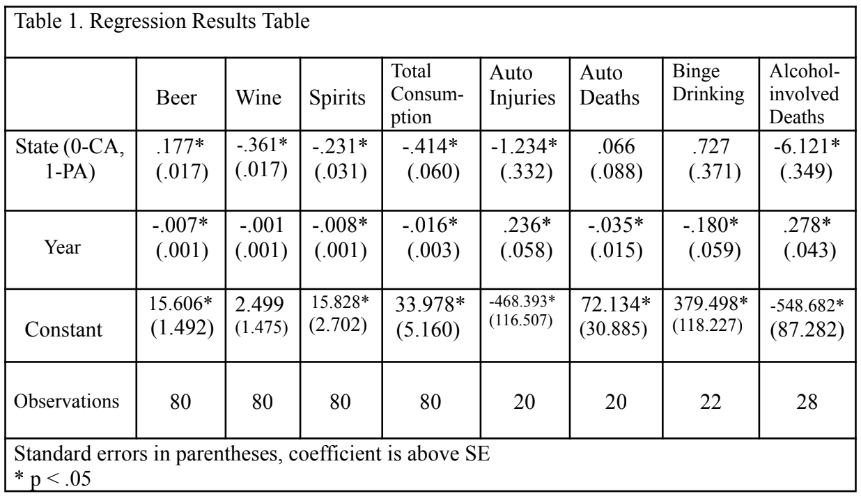
In this table, the far left column has three categories (Year, Constant, and Observations) that do not concern the results of this analysis. The reason for “Year” standing as a controlled variable was to make sure that time is not what is explaining these effects. “Constant” and “Observations” do not have any meaningful interpretation for the analysis. The category that is important in determining the results is the “State (0-CA, 1-PA)” variable. The remainder of the columns in the table are the dependent variables with their coefficients, indicators of significance, and standard error from the regression analysis.
The first dependent variable on the table is per capita beer consumption. The coefficient is positive (.177), and the p-value is less than .05 (p<.001), meaning that the relationship is statistically significant. As mentioned previously, due to the state variable being coded as 0=CA and 1=PA, it is interpreted that its effect as moving from CA to PA. Due to the direction of the coefficient being positive, it is interpreted that this as meaning moving from CA to PA increases the per capita consumption of beer. In other words, Pennsylvania’s beer consumption per capita is significantly higher than California’s. The original hypothesis for beer consumption predicted that there would be no difference between the two states, however, Pennsylvania has higher rates of beer consumption, therefore the original hypothesis is rejected.
The second, third, and fourth columns depict the next three dependent variables: per capita wine consumption, per capita spirits consumption, and per capita consumption of all types of alcohol (sum of beer, wine, and spirits). Wine, spirits, and total alcohol consumption all have negative coefficients with p-values of less than .05 (<.001 for all three). Therefore, the relationship between the independent variable and these three dependent variables is statistically significant. Due to the direction of the coefficients for these three variables being negative, it is interpreted that this means moving from CA to PA decreases per capita wine, spirits, and total alcohol consumption. In other words, California has significantly higher rates of wine, spirits, and total alcohol consumption. The original hypotheses for these variables predicted that California would have higher rates for all three, thus confirming these hypotheses.
In the fifth column of the table, the variable is the number of serious injuries in alcohol-related car crashes per 100,000 people. This variable has a negative coefficient (-1.243) with a p-value of less than .05 (p=.002). This relationship is statistically significant, and the direction is negative, which tells us that California has significantly higher rates of serious injuries from alcohol-related car crashes. The original hypothesis for this variable predicted that California would have higher rates, therefore confirming the hypothesis. The sixth and seventh column of the table shows the variables of the number of fatalities in alcohol-related car crashes per 100,000 people and binge drinking (percent of adults consuming at least 4 (women) or 5 (men) drinks on one occasion in the last 30 days). The coefficient for the crash fatalities variable is positive (.066), and the p-value is not less than .05 (.463). This means that the relationship between the independent and dependent variables is insignificant. Therefore, there is no difference between California and Pennsylvania in regard to the number of fatalities in alcohol-related car crashes. The coefficient for the binge drinking variable is positive (.727), and the p-value is not less than .05 (p=.065). There is also no statistically significant relationship, therefore, there is no difference between California and Pennsylvania binge drinking rates. The original hypothesis for these two variables predicted that California would have higher rates for both; however, this is not the case; therefore, the original hypothesis for these variables is rejected.
The final variable in the table that was tested is the number of alcohol-related deaths per 100,000 people. The coefficient for this variable is negative (-6.121), and the p-value is less than .05 (p<.001). This means that this relationship is statistically significant, and the coefficient being negative shows that California has significantly higher rates of alcohol-involved deaths. It was initially predicted that California would have greater numbers of deaths involving alcohol, and this was proven to be correct.
Discussion & Conclusion
Overall, based on the findings of the regression analysis, it is clear that California has greater rates of alcohol-related harm than Pennsylvania. This confirms the original prediction for this study that California would have greater rates because alcohol is more widely accessible than it is in Pennsylvania. California has more total alcohol consumption per 100,000 people, higher rates of injuries from alcohol-related crashes, and more alcohol-involved deaths per 100,000. Pennsylvania has more beer consumption than California, but this is not surprising, and it is most likely due to the fact that it is the least regulated type of alcohol; therefore, it is more popular than others. There were no differences between both states in regards to binge drinking and fatalities from alcohol-related crashes. This was a surprising finding, and there could be numerous reasons for it. It warrants further research as to why there are no differences for these two alcohol-related harms. However, there are dramatic differences in others, like serious injuries from alcohol-related crashes.
Future research should also analyze more state-to-state comparisons. It would be very interesting to see if two different states, both with very different alcohol laws, are compared and produce results similar to this analysis. This would provide further evidence that shows the impact that alcohol laws have on public health in regard to preventing alcohol-related harms. Using more dependent variables for future research could also be helpful in determining the effects of alcohol laws on public health. Examples of other dependent variables that could be used are: underage drinking rates, the economic impact of alcohol abuse, and the health consequences of excessive consumption.
This study contributes to this overall field of research by directly comparing two states with very different alcohol policies and determining through statistical analysis which set of laws best impacts public health. This research, when comparing PA and CA, found that Pennsylvania typically has less alcohol consumption, fewer serious injuries from alcohol-related car crashes, and fewer alcohol-involved deaths. Therefore, it may be said that Pennsylvania’s strict alcohol laws have a better overall impact on public health than the state of California. These findings raise concerns about those states that have more lenient alcohol laws similar to California. The data clearly shows that more alcohol regulations play a large role in decreasing the number of alcohol-involved fatalities and harms in a state’s population. California and states that have similar alcohol laws should consider increasing alcohol restrictions in order to better public health and save lives from alcohol-related harms.
References
“Bar: Alcohol-Involved Deaths per 100,000 People: State Health Access Data Assistance Center.” Bar | Alcohol-Involved Deaths per 100,000 People | State Health Access Data Assistance Center, https://statehealthcompare.shadac.org/bar/269/alcoholinvolved-deaths -per-100000-people# 0/6,40/a/27/305.
Baughman, Reagan Anne, et al. “Slippery When Wet: The Effects of Local Alcohol Access Laws on Highway Safety.” SSRN Electronic Journal, 2001, https://doi.org/10.2139/ssrn.275157.
“California Population 1900-2022.” MacroTrends, https://www.macrotrends.net/states/california/ population.
“California.” National Institute on Alcohol Abuse and Alcoholism, U.S. Department of Health and Human Services, https://alcoholpolicy.niaaa.nih.gov/underage-drinking/state-profiles/ california/56#:~:text=Underage%20Drinking%3A%20Underage%20Possession%20of,OR%20spouse.
Campbell, Carla Alexia, et al. “The Effectiveness of Limiting Alcohol Outlet Density as a Means of Reducing Excessive Alcohol Consumption and Alcohol-Related Harms.” American Journal of Preventive Medicine, vol. 37, no. 6, 2009, pp. 556–569., https://doi.org/10. 1016/j.amepre.2009.09.028.
“Code Section Group.” Codes Display Text, https://leginfo.legislature.ca.gov/faces/codes_display Text.xhtml?lawCode=BPC&division=9.&title=&part=&chapter=16.&article=3.
“Code Section Group.” Codes Display Text, https://leginfo.legislature.ca.gov/faces/codes_display Text.xhtml?lawCode=BPC&division=9.&title=&part=&chapter=16.&article.
Hadley, Carrie. “Prohibition’s Legacy in Pennsylvania.” Heinz History Center, Heinz History Center, 14 Dec. 2022, https://www.heinzhistorycenter.org/blog/western-pennsylvania- history-prohibitions-legacypennsylvania/.
Identification Information – Pennsylvania Liquor Control Board. https://www.lcb.pa.gov/Legal/ Documents/000812.pdf.
Naimi, Timothy S., et al. “A New Scale of the U.S. Alcohol Policy Environment and Its Relationship to Binge Drinking.” American Journal of Preventive Medicine, vol. 46, no. 1, 2014, pp. 10–16., https://doi.org/10.1016/j.amepre.2013.07.015.
Ornstein, Stanley I., and Dominique M. Hanssens. “Alcohol Control Laws and the Consumption of Distilled Spirits and Beer.” Journal of Consumer Research, vol. 12, no. 2, 1985, pp. 200–13. JSTOR, http://www.jstor.org/stable/254353.
Pennsylvania Crash Information Tool, https://crashinfo.penndot.gov/PCIT/welcome.html. “Pennsylvania Population 1900-2022.” MacroTrends, https://www.macrotrends. net/states/pennsylvania/population#:~:text=The%20population%20of%20Pennsylvania %20in%202021%20was%2013%2C012%2C059%2C%20a%200.14 ,a%200.08%25% 20decline%20from%202018.
“Pennsylvania.” National Institute on Alcohol Abuse and Alcoholism, U.S. Department of Health and Human Services, https://alcoholpolicy.niaaa.nih.gov/underage-drinking/state-profiles /pennsylvania/90.
“Publications.” National Institute on Alcohol Abuse and Alcoholism, U.S. Department of Health and Human Services, https://pubs.niaaa.nih.gov/publications/surveillance110/tab4- 1_16.htm. State of California. “Minors.” Alcoholic Beverage Control, https://www.abc.ca.gov/education/merchant-education/on-sale-licensee-informational-guid e/minors/.
“Table: Percent of Adults Consuming Four (Women) or Five (Men) or More Drinks on One Occasion during the Past 30 Days by Total (2011 to 2021): State Health Access Data Assistance Center.” Table | Percent of Adults Consuming Four (Women) or Five (Men) or More Drinks on One Occasion during the Past 30 Days by Total (2011 to 2021) | State Health Access Data Assistance Center, https://statehealthcompare.shadac.org/table /40/percent-of-adults-consuming-four-women-or-five-men-or-more-drinks-on-one-occasion-during-the-past-30#6,40/a/32/71.
“Table: Percent of Adults Consuming Four (Women) or Five (Men) or More Drinks on One Occasion during the Past 30 Days by Total (2011 to 2021): State Health Access Data Assistance Center.” Table | Percent of Adults Consuming Four (Women) or Five (Men) or More Drinks on One Occasion during the Past 30 Days by Total (2011 to 2021) | State Health Access Data Assistance Center, https://statehealthcompare.shadac.org/table/40/ percent-of-adults-consuming-four-women-or-five-men-or-more-drinks-on-one-occasion-during-the-past-30#6,40/a/32/71.
“Transportation Injury Mapping System.” TIMS, https://tims.berkeley.edu/summary.php.
Vadala, Nick. “Pennsylvania’s Weird Liquor Laws, Explained.” The Philadelphia Inquirer, 13 July 2021, https://www.inquirer.com/philly-tips/pennsylvania-liquor-laws.html.